Expand
When perfect effectiveness cannot be assumed, the assessment of hedge effectiveness will be more complex – an initial quantitative “long-haul” analysis of hedge effectiveness will be required.

9.11.1 Reasons an initial quantitative test would be needed

There are many reasons why a hedge might not be perfectly effective, and therefore, an initial quantitative test might be required and an entity would recognize some volatility in net income during the life of the hedge (for a fair value hedge) or when the hedged item and derivative impact earnings (for a cash flow or net investment hedge).
Circumstances that may preclude a reporting entity from assuming perfect effectiveness at inception of the hedging relationship include:
  • A difference between the basis of the hedging instrument and the hedged item or transaction, such as:
    • A LIBOR-based derivative versus a financial instrument with a contractually specified interest rate based on the prime rate
    • Differences in SOFR calculation methodologies between the hedged item and the derivative
    • An Australian dollar-denominated hedging instrument and a New Zealand dollar-denominated hedged item

      Cross-currency hedging is broadly permissible under ASC 815-25-55-3; however, practically, it may be difficult to prove that the hedge is highly effective 2.
    • An aluminum-based derivative and a manufactured product whose principal raw material is aluminum, but the aluminum price component is either (1) not contractually specified or (2) is contractually specified based on a different index than the derivative
  • Differences in the critical terms of the hedging instrument and hedged item or transaction, such as differences in the principal and notional amounts, rate reset dates, the term or maturity, or cash receipt or payment dates (beyond the 31 days or same fiscal month permitted for certain hedges per ASC 815-20-25-84A)

2ASC 815-25-55-3 indicates that the use of a hedging instrument with a different underlying basis than the item or transaction being hedged is referred to as a cross hedge. The principles for assessing the effectiveness of cross-hedges illustrated in the guidance also apply to hedges involving other risks. For example, the effectiveness of a hedge of interest rate risk in which one interest rate is used as a surrogate for another would be evaluated in the same way as it is for the cross-hedge.
  • Location differences between the commodity on which the derivative’s underlying is based and the location of the commodity actually being purchased or sold (when hedging the total cash flows or total change in fair value)
  • Hedging relationships using purchased options when the provisions of ASC 815-20-25-128 have not been utilized and time value is not excluded from the assessment of effectiveness
  • Forward premiums or discounts that represent the cost of the derivative that are not excluded from the assessment of effectiveness (e.g., a foreign currency spot transaction hedged with a forward foreign exchange contract)
  • When the payment dates of the hedged assets differ in a portfolio layer method hedge

    Although the guidance in ASC 815-20-55-14A permits a qualitative similar assets test in a last-of-layer hedge, the assessment of effectiveness may not be able to be performed qualitatively. See DH 6.5.
  • Use of different discount rates in a fair value hedge of benchmark interest rate risk when the shortcut method is not applied

    For example, when designating a fair value hedge of a fixed-rate financial instrument for changes in fair value due to changes in the benchmark interest rate using an interest rate swap, the change in value of the hedged item (or benchmark component of the hedged item) attributable to changes in the benchmark interest rate must be discounted using the benchmark interest rate. However, the fair value of the swap could be impacted by other valuation adjustments (e.g., own and counterparty credit risk, using overnight index swap (OIS) or OIS-based discount rates for collateralized positions).
As a general rule, these or other mismatches in a hedging relationship should be identified in the hedge documentation and assessed as to their potential impact on effectiveness at inception and in subsequent assessments of effectiveness.
However, if an initial quantitative assessment is performed, the subsequent prospective and retrospective assessments of effectiveness may be performed qualitatively if certain conditions are met. A reporting entity may make the election either to perform subsequent effectiveness assessments qualitatively or quantitatively on a hedge-by-hedge basis.
At inception of the hedging relationship, a reporting entity is required by ASC 815-20-25-3(b)(2)(iv)(03) to document whether it elects to perform subsequent retrospective and prospective hedge effectiveness assessments on a qualitative basis and how it intends to carry out the qualitative assessment. The guidance also requires that the entity document which quantitative method it will use if the facts and circumstances of the hedging relationship change and the entity must quantitatively assess hedge effectiveness. The subsequent ongoing prospective quantitative effectiveness assessment method must be the same as the prospective quantitative effectiveness assessment method used at hedge inception.
As specified in ASC 815-20-35-2A, a reporting entity may qualitatively assess hedge effectiveness after hedge inception only if it:
  • performs an initial quantitative test of hedge effectiveness on a prospective basis that demonstrates that the hedging relationship is highly effective, and
  • can reasonably support at hedge inception an expectation of high effectiveness on a qualitative basis in subsequent periods.
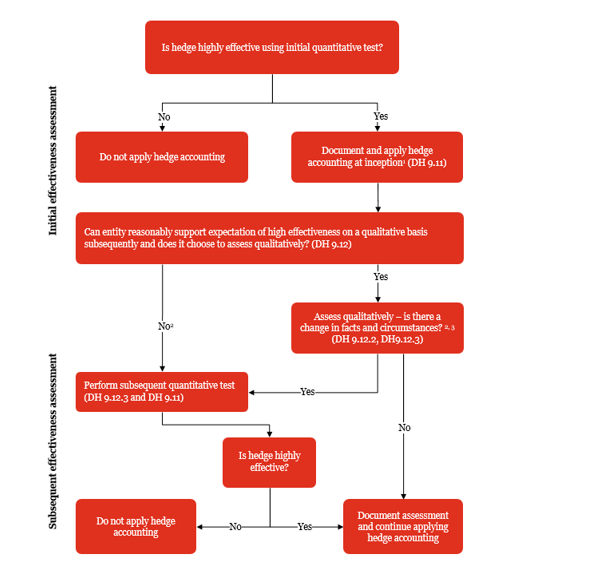
Figure DH 9-3 summarizes effectiveness requirements when the hedging relationship is not assumed to be perfectly effective (i.e., an initial quantitative test is required). It is the same as Figure DH 9-1 without the decision tree relating to an assumption of perfect effectiveness.
Figure DH 9-3
Effectiveness requirements when hedge is not assumed to be perfectly effective
View image
1Assuming other qualifying criteria are met
2If there is an adverse change in the risk of default, reporting entities should consider the need to dedesignate the hedging relationship.
3A reporting entity may choose to perform a quantitative assessment at any time. It may then revert to a qualitative assessment subsequently if it can reasonably support an expectation of high effectiveness on a qualitative basis for subsequent periods.
Long-haul quantitative methods commonly accepted under ASC 815-20-25-3 include dollar-offset or a statistical method, such as regression analysis. While ASC 815-20-25-79 provides for choice of method, we have observed that the general practice has been to elect a regression approach for both the required prospective testing (at inception and on an ongoing basis, as applicable) and retrospective testing (on an ongoing basis, as applicable), discussed in DH 9.2.2.
Long-haul methods are also generally available for purposes of assessing hedge effectiveness when one of the methods detailed in Figure DH 9-2 in which perfect effectiveness can be assumed (such as the shortcut method or critical terms match approach) is allowed. Because of some of the nuances in eligibility of these approaches and the consequences of incorrect application, reporting entities might want to consider application of one of the long-haul methods if they are uncertain as to whether they qualify and will continue to qualify for an assumption of perfect effectiveness.
ASC 815-25-55 and ASC 815-30-55 describe several (but not all) acceptable and unacceptable methods of assessing effectiveness for specific fair value and cash flow hedges.
In determining how effectiveness should be assessed, reporting entities should consider how they have defined the hedged risk and any excluded components (discussed in DH 9.3.3). Both the hedged risk and excluded components may have a significant impact on how the hedged item or transaction is modeled in quantitative assessments of effectiveness and the ability to qualify for qualitative subsequent testing.

9.11.2 Portfolio layer method hedges

Given how the portfolio layer method (discussed in DH 6.5) works, many aspects of the effectiveness assessment will be simplified when the portfolio layer method is used.
  • If the hedged item is designated using the partial-term guidance (i.e., the hedge period is for some portion of the term of the asset), the remaining term of all assets in the portfolio may be the same (as each other) for hedge accounting purposes.
  • Prepayments do not need to be considered in measuring the hedged item in a portfolio layer method hedge because what is being hedged is a portion of the portfolio that will remain throughout the assumed maturity of the portfolio.
Although prepayments do not need to be considered in measuring the hedged item, differences in payment dates among the assets in the closed portfolio and the derivative hedging instrument need to be considered in the assessment of effectiveness and may invalidate the assumption of perfect effectiveness since the benchmark component of the coupon cash flows on the closed portfolio (the hedged item) and hedging instrument will differ, creating a difference in the measurement of the derivative and the hedged item in earnings. The guidance in ASC 815-20-55-14A contemplates a qualitative similar assets test but that does not mean that the assessment of effectiveness can be performed qualitatively. Additionally, if a reporting entity chooses not to use the benchmark component of the contractual cash flows, the different contractual coupon rates (if any) among the assets in the closed portfolio would need to be incorporated into the similar asset analysis and the effectiveness assessment.

9.11.3 Modelling hedged cash flows

In certain situations, it may be difficult for a reporting entity to calculate the change in fair value (or present value of cash flows) of the hedged portion of the hedged item. ASC 815 permits several methods to model the hedged cash flows.

9.11.3.1 Hypothetical derivative method

When applying a quantitative method to assess effectiveness in a cash flow hedging relationship, many reporting entities determine the change in fair value of the hedged cash flows by using a perfectly effective hypothetical derivative, i.e., a derivative with terms that match those of the hedged item and would therefore represent the “perfect” derivative for the hedged risk. The reporting entity compares the change in fair value of the hypothetical derivative to the change in fair value of the hedging instrument in assessing whether the hedge is highly effective.
The term “hypothetical derivative” is used within ASC 815-30-35-25 through ASC 815-30-35-29, which provides guidance on assessing effectiveness for hedges using interest rate swaps. However, the concept of a hypothetical derivative is used more broadly in practice for cash flow hedges because it provides a basis for comparison when determining whether a hedging instrument is highly effective. A hypothetical derivative may be used for options, forwards, swaps, or other derivatives and for other exposures in addition to interest rate risk (e.g., foreign currency or commodity price risk).
The perfect hypothetical derivative is a derivative that has terms that are identical to the critical terms of the hedged item and has a fair value of zero at inception of the hedging relationship. As indicated in ASC 815-20-55-108 through ASC 815-20-55-109, if an entity uses the hypothetical derivative method and determines that the terms of the hypothetical derivative exactly match the terms of the actual hedging instrument, the actual swap would be expected to perfectly offset the hedged cash flows. In these cases, we do not believe an initial quantitative assessment test is required, based on the guidance in ASC 815-20-25-3(b)(2)(iv)(01)(F).
We recommend that the reporting entity still specify and document at inception of the hedging relationship a long-haul approach using the hypothetical derivative method to ensure that if the terms of the forecasted transaction change, the reporting entity will not automatically have to dedesignate the hedging relationship because the terms of the actual and hypothetical derivatives differ. Under this approach, the reporting entity could document that an initial quantitative test was not required since the actual derivative was equal to the hypothetical derivative. However, if the terms do not exactly match, a quantitative assessment is needed to determine if the hedge is effective.
The determination of the fair value of both the perfect hypothetical derivative and the actual derivative should use discount rates based on the relevant swap curves.
In some cases, use of the hypothetical derivative method to assess effectiveness is required, including:
For net investment hedges, ASC 815-35-35-11, ASC 815-35-35-14, ASC 815-35-35-19, and ASC 815-35-35-20 specify that the hypothetical instrument used to assess hedge effectiveness should have a maturity and repricing and payment frequencies for any interim payments that match those in the actual designated hedging instrument in the net investment hedge.

9.11.3.2 Change-in-variable-cash-flows method

A reporting entity may also use the change-in-variable-cash-flows method to assess effectiveness of a cash flow hedge in certain circumstances. See DH 9.7 for more information.

9.11.3.3 Change-in-fair-value method

When applying a quantitative method to assess effectiveness in a cash flow hedging relationship, reporting entities may also determine the change in fair value of the hedged cash flows by using the change-in-fair-value method, discussed in ASC 815-30-35-31.
Under the change-in-fair-value method, the assessment of hedge effectiveness is based on a calculation that compares the present value of (1) the cumulative change in expected variable future cash flows that are designated as the hedged transactions and (2) the cumulative change in the fair value of the derivative hedging instrument. The present values of the cumulative changes in the hedged cash flows should be discounted by the rate used to determine the fair value of the swap.
An entity must also assess the risk of counterparty default as required by ASC 815-20-25-122. If the likelihood of the obligor defaulting is assessed as being probable, the hedging relationship would not qualify for hedge accounting.

9.11.4 Quantitative methods of assessing effectiveness

The most common quantitative methods for assessing hedge effectiveness are dollar-offset and regression analysis, but other methods may also be appropriate.

9.11.4.1 Dollar-offset analysis

The dollar-offset method compares the change in fair value or present value of cash flows of the hedging instrument to the changes in the fair value or present value of cash flows of the hedged item. The dollar-offset method can be used in performing the prospective and/or the retrospective assessments of effectiveness. This is supported by ASC 815-20-35-12.

Excerpt from ASC 815-20-35-12

… the entity must assess whether the hedging relationship is expected to continue to be highly effective using a quantitative assessment method (either a dollar-offset test or a statistical method such as regression analysis).

As discussed in ASC 815-20-35-5, there are two permissible methods for retrospective assessments of effectiveness under a dollar-offset approach: (1) the discrete (or period-by-period) approach and (2) the cumulative approach. As their names imply, the discrete method computes an effectiveness ratio based on the changes occurring in the period being assessed, while the cumulative method computes an effectiveness ratio based on the cumulative change since inception of the hedge.
Figure DH 9-4 illustrates the discrete and cumulative approaches.
Figure DH 9-4
Dollar offset: discrete and cumulative approaches
Dollar-offset analysis
End of
Derivative
Change 1
Hedged item
Change 2
Discrete
Cumulative
Inception
$0
$0
$0
$0
Quarter 1
50
50
(50)
(50)
100%
100%
Quarter 2
105
55
(107)
(57)
96%
98%
Quarter 3
129
24
(120)
(13)
185%
108%
Quarter 4
115
(14)
(116)
4
350%
99%
View table
1Represents the change in fair value of the derivative.
2 Represents either the change in (1) fair value or (2) present value of the expected future cash flows of the hedged item.
As Figure DH 9-4 demonstrates, using the discrete period method of assessing effectiveness results in disqualification of the hedge in quarters 3 and 4 (when the hedge effectiveness ratio is outside of the 80%-125% threshold), and thus, the inability to apply hedge accounting in those quarters.
If the cumulative method had been used, all periods would have been considered highly effective (within the 80%-125% threshold) and the hedging relationship would have qualified for hedge accounting.
When using the dollar-offset method, a reporting entity is free to select either the cumulative or the discrete method when assessing hedge effectiveness; but once selected, it must abide by the results regardless of the outcome, as discussed in ASC 815-20-35-6. A different method of assessing hedge effectiveness may never be selected in hindsight.
Advantages/disadvantages to dollar-offset
While the dollar-offset method is simple to understand and easy to implement, its use might result in difficulties demonstrating high effectiveness for the hedging relationship, particularly when there are isolated periods of aberration in the behavior of the underlying. Generally, hedging relationships that contain basis differences have an elevated risk of not qualifying for hedge accounting under a retrospective test because such an aberration could weigh heavily in the assessment results.
An example of aberrant behavior is when there is a period of low price volatility in the principal underlying reflected in the hedging instrument such that the changes in the fair value or present value of cash flows of the hedging instrument and the hedged item are small. While many hedging relationships will pass a dollar-offset test for high effectiveness when there are reasonably sized movements in the price of the principal underlying, it is not uncommon for them to fail when there is a small movement. This is because the difference will potentially represent a far greater portion of the overall change in the hedged item. For example, assume a fair value hedge in which the notional amount of the hedged item and the derivative are each $100 million. If the fair value of the hedged item changes by $500,000 over the assessment period and the change in the fair value of the hedging instrument is within plus or minus 10% of the change in the fair value of the hedged item, the dollar-offset ratio would be 1.1 (i.e., $550,000 divided by $500,000). However, if in a period of low volatility for the underlying, the change in fair value of the hedging instrument was $65,000, and the change in fair value of the hedged item is $50,000, the dollar-offset ratio would be 1.3 and the hedging relationship would fail the effectiveness assessment.
Because of the risk of losing hedge effectiveness in periods of low volatility, many reporting entities use regression analysis instead of the dollar-offset approach. Regression analysis evaluates the relationship between the hedging instrument and the hedged item over a number of periods, and thus, isolated periods of low volatility in the underlying will generally not cause the hedge to fail the effectiveness test.

9.11.4.2 Regression analysis

Regression analysis is a statistical technique used to analyze the relationship between one variable (the dependent variable) and one or more other variables (independent variables) using a set of data points. A regression model is a formal means of expressing a tendency of the dependent variable to vary with the independent variable in a systematic fashion.
In the context of a hedge effectiveness assessment, the primary objective of regression analysis is to determine if changes to the hedged item and derivative are highly correlated and, thus, supportive of the assertion that there will be a high degree of offset in fair values or cash flows achieved by the hedge. For example, if a $10 change in the dependent variable (i.e., the derivative) was accompanied by an offsetting $10.01 change in the independent variable (i.e., the hedged item) and if further changes in the dependent variable were accompanied by similar magnitude changes in the independent variable, there would be a strong correlation because approximately 100% of the change in the dependent variable can be “explained” by the change in the independent variable.
The use of regression analysis is more likely than the dollar-offset method to enable a reporting entity to continue with hedge accounting despite unusual aberrations that may occur in a particular period. The application of regression analysis allows isolated aberrations to be minimized by more normal changes in fair value that occur over the remainder of the periods included in the regression. However, the use of regression analysis is complex; it requires considerable effort to develop the models, and interpreting the results requires judgment.
Model inputs
The following are key considerations regarding inputs in the regression analysis.
Dependent and independent variables
In the regression model, the change in fair value of the derivative will likely be the dependent variable (Y) and the change in fair value of the hedged item will likely be the independent variable (X).
Data points
The objective of the regression analysis is to estimate a linear equation that best captures the relationship between the hedged item and the derivative. The inputs are a series of matched-pair observations for the hedged item and derivative. For example, the inputs could be the change in fair value of the hedged item and derivative observed weekly between January 1, 20X1 and October 31, 20X1. Thus, the first observation would be as of January 8, 20X1 and would include only the changes in the fair value of the derivative and the hedged item from January 1, 20X1 to January 8, 20X1. Subsequent observations would include only the changes in the fair value of the derivative and hedged item that occur during the weekly periods under observation (i.e., not on a cumulative basis). Use of cumulative changes has a propensity to create autocorrelation in the regression analysis, which may invalidate it. See the Other considerations section later in this section.
In calculating the data points to be used in the regression model, reporting entities should also decide whether to use a declining maturity approach (i.e., the remaining term of the hedged item and hedging instrument will vary at each data point because the maturity date is held constant) or a constant maturity approach (i.e., the remaining term of the hedged item and hedging instrument will stay constant at each data point).
  • In a declining maturity approach, the reporting entity uses some previously-calculated data points by removing the oldest and adding more recent data points (keeping the number of data points the same each period).
  • In a constant maturity approach, all of the data points are recalculated in each successive analysis as the remaining tenor or life of the derivative changes over time.
Time horizon
For prospective considerations throughout the life of a hedging relationship, the analysis should use observations selected on a consistent basis over a consistent period of time. The time horizon (period over which data points are gathered) should be relevant for the hedging period and statistically significant.
Number of data points
It is important to use a sufficient number of data points to ensure a statistically valid regression analysis. Generally speaking, as sample size increases, interpretation of the model and conclusions that can be drawn improve. We expect most regression analyses conducted to assess hedge effectiveness will be based on 30 or more observations, but fewer may be acceptable in certain circumstances.
ASC 815-20-35-3 permits a reporting entity to use the same regression analysis for both prospective and retrospective tests. The regression calculations should use the same number of data points, and the reporting entity must periodically update the data points used in its regression analysis.
Results
The following are the key metrics in a statistically-significant regression analysis.
  • The R 2 statistic should be 80% (.8) or greater.
  • The slope coefficient should be between -0.8 and -1.25.
  • The F-statistic or t-statistic associated with the slope coefficient should be significant at a 95% or greater confidence level.
In addition:
  • Unexpectedly large residuals, especially recent ones, may indicate an unusual period in the relationship.
  • The possibility of autocorrelation should be considered.
R 2
The degree of explanatory power or correlation between the dependent and independent variables is measured by the coefficient of determination, or R 2. R 2 is one of the key statistical considerations when a regression analysis is used to support hedge accounting. The R 2 indicates the portion of variability in the dependent variable that can be explained by variation in the independent variable. Therefore, the higher the R 2 for a hedging strategy, the more effective the relationship is likely to be.
Although ASC 815 does not provide a specific threshold for R 2, practice generally requires an R 2 of 0.80 or higher for a hedging relationship to be considered highly effective.
While the R 2 is a key metric, it is not the only consideration when using regression analysis to evaluate the effectiveness of a hedging relationship. Reporting entities should also evaluate the slope coefficient and the F-statistic or t-statistic, the statistical significance of the relationship between the variables.
Slope coefficient
The slope is an important component of a highly effective hedging relationship. The slope coefficient is the slope of the straight line that the regression analysis determines "best fits" the data.
Many regression analyses uses the "least squares" method to fit a line through the set of observations (ordinary least squares regression). This method determines the intercept and slope that minimize the size of the squared differences between the actual Y observations and the predicted Y values (i.e., the vertical differences between plotted observations and the regression line).
The slope coefficient should be interpreted as the change in the derivative associated with a change in the hedged item. If the model is developed using the change in fair value of the derivative as the dependent variable (Y) and the change in fair value of the hedged item the independent variable (X), the slope equals the change in Y divided by the change in X, or "rise" over "run." In effective 1 for 1 hedging relationships, the slope coefficient will approximate a value of -1. In practice, many reporting entities apply a range of -0.80 to -1.25, as described in DH 9.2.1.
The slope coefficient should be negative (except when the hedged item is represented by a hypothetical derivative in a cash flow hedge) because the derivative is expected to offset changes in the hedged item. In other words, to be an effective hedging relationship, the derivative and the hedged item must move in an inverse manner. If the analysis yields a positive slope coefficient, it means that when the hedged item goes up in value, the derivative goes up in value, which is not a hedge. If the hypothetical derivative method is used in a regression as a proxy for the hedged item, the slope of a regression line would be positive, since the actual derivative is compared to a hypothetical derivative, rather than to the hedged item itself.
F-statistic or t-statistic
An F-statistic or t-statistic associated with the slope coefficient is useful in determining whether there is a statistically significant relationship between the dependent and independent variables. In ordinary least squares regression analyses, the F-statistic is equal to the squared t-statistic for the slope coefficient. Generally, the result should be significant at a 95% confidence level.
Other considerations
Unexpectedly large residuals (relative to the predicted value or to other residuals) may indicate an unusual period in the relationship between the dependent and independent variables. In many cases when the regression analysis yields acceptable results, the residuals will not be important. However, residuals may signal declining effectiveness if the largest residuals come primarily from the most recent observations. Judgment should be used when interpreting declining effectiveness over time. The decline could be temporary, or it could call into question the effectiveness of the hedging relationship in future periods if the trend persists.
One of the assumptions underlying ordinary least squares regression is that the errors are uncorrelated. Correlated errors are referred to as “autocorrelation.” Autocorrelation may indicate that the regression model is not statistically valid because it can cause the R 2, F-statistic (or t-statistic), and slope coefficient to be misstated. In time series data, autocorrelation can be caused by the prolonged influence of shocks in the economy (e.g., the effects of war or strikes can affect several periods). Autocorrelation can also be artificially induced through the use of overlapping observations. For example, overlapping inputs would result if the first observation in a regression analysis is the change in value from January 1, 20X1 to March 31, 20X1 and the second observation is the change in value from February 1, 20X1 to April 30, 20X1. The use of overlapping inputs creates a dependency in the input variables because some months of each observation are the same, and should be avoided.
Reporting entities should consider use of statistical procedures that are available to detect, and attempt to correct for, autocorrelation, such as the Durbin-Watson Test.
Expand Expand
Resize
Tools
Rcl

Welcome to Viewpoint, the new platform that replaces Inform. Once you have viewed this piece of content, to ensure you can access the content most relevant to you, please confirm your territory.

signin option menu option suggested option contentmouse option displaycontent option contentpage option relatedlink option prevandafter option trending option searchicon option search option feedback option end slide