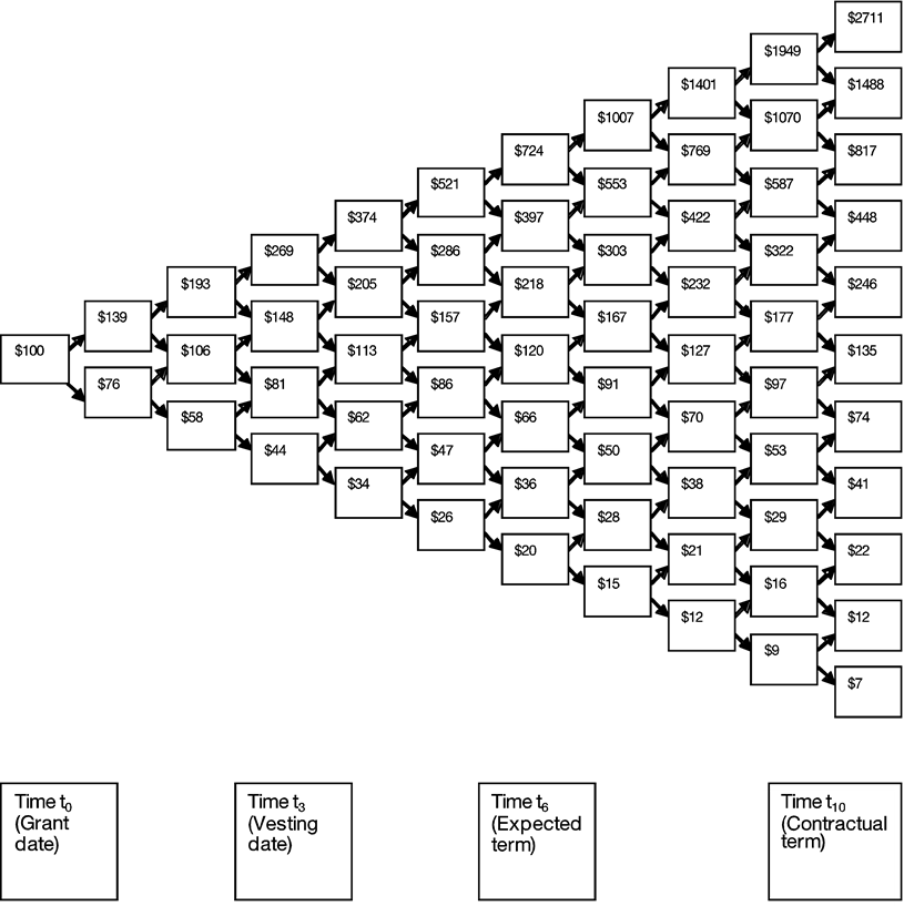
The example in Figure SC 8-7 still assumes a single value for the expected term of the option rather than the more varied employee exercise behavior that would occur in reality, which may include the correlation between possible stock price appreciation and the expected time of exercise. However, the main reason to use a binomial model is to incorporate such assumptions over the option's contractual term. Because complex exercise pattern assumptions are not reflected in Figure SC 8-7, the estimates of fair value produced by the Black-Scholes model and the simplified binomial model will converge given a sufficient number of nodes.

One method to incorporate early-exercise behavior assumes exercises based on stock price appreciation. As mentioned previously, a lattice model would simulate exercise behavior over the entire contractual term, rather than simply using the single average expected term as illustrated in Figure SC 8-7. Figure SC 8-8 shows another option valuation binomial tree-diagram, in which exercise is assumed to occur whenever the stock price reaches $200 (i.e., the stock to exercise price multiple of 2.0 is a "threshold" at which exercise is assumed to occur at a date prior to the end of the contractual term). The option value tree-diagram now covers the entire 10-year contractual life of the option instead of the six-year expected term as in Figure SC 8-7, since the option values must be simulated over the contractual life of the option in case the assumed exercise multiple is not reached. At time t₁₀ (the end of the option's contractual life), the option is assumed to be exercised immediately if it has any intrinsic value at that point. If the stock price is less than the exercise price at time t₁₀, the option expires worthless (i.e., the value is zero).

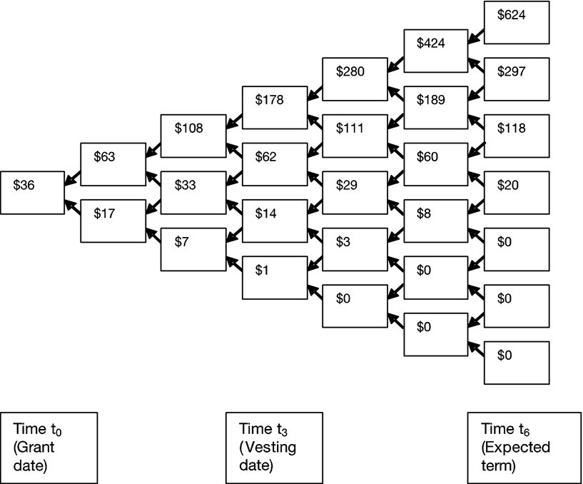
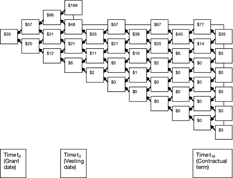
Figure SC 8-8
Option tree—ten-year contractual term with a 2.0 assumed exercise multiple

View image

The values along the top boundary in Figure SC 8-8 will equal the option's intrinsic value (the greater of the stock price minus $100, or zero), similar to the values at time t₆ in Figure SC 8-7. This boundary may be thought of as the "exercise frontier" (i.e., the points along the price-time continuum at which exercise is assumed to occur). As exercise is assumed to occur at these boundary points, no nodes above that line are necessary. The calculation proceeds "backwards" from the terminal values using risk-neutral probabilities and discounting for the time value of money. While the time-horizon imposed by the option's 10-year contractual life is reflected in this example, the constraint imposed by the three-year cliff vesting assumption has no effect because the highest potential stock-price at time t₂ (the last node before vesting in our simple one step per year example) is $193, which is less than the assumed exercise threshold of $200. Refer to the corresponding node in Figure SC 8-6, which illustrates the potential stock prices; the values in Figure SC 8-8 above represent potential option-values.

The calculation shown in Figure SC 8-8 results in a fair value of approximately $42 or 17% higher than the approximately $36 fair-value (based on the static six-year expected term) from Figure SC 8-7. The use of an early-exercise assumption (i.e., the single average six-year expected term) will generally reduce the estimated fair value of an option as compared to a model that considers the full contractual life of ten years (on other than a dividend-paying stock, which can make it advantageous to exercise early in some circumstances). However, depending on where the assumed exercise multiple is set when exercise behavior is modeled based on stock-price appreciation, an option's fair value could be higher or lower than that of an otherwise similar option with an assumed static expected term.

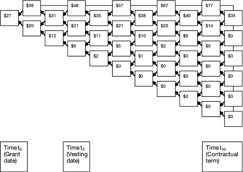
To explore the relationship between this type of early-exercise assumption and an option's fair value, Figure SC 8-9 presents another example, identical to the scenario presented in Figure SC 8-8, except that exercise is assumed to occur whenever the price of the underlying stock reaches $130 (i.e., when the assumed exercise multiple reaches 1.3).

Figure SC 8-9
Option tree—ten-year contractual term with a 1.3 assumed exercise multiple

View image

The calculations in Figure SC 8-9 result in a fair value of approximately $27, 36% lower than the fair value of approximately $42, calculated in Figure SC 8-8 (using an assumed exercise multiple of 2.0). This dramatic decrease shows the sensitivity of fair value to the assumed exercise multiple—by essentially truncating the model for significantly more valuable payouts by using a lower exercise multiple, the fair value of the award is much lower. However, the calculation in Figure SC 8-9 may require further adjustment to reflect the terms and conditions of the award. Specifically, the exercise frontier shown in Figure SC 8-9 includes potential exercise scenarios as early as one year after grant (i.e., at a price of $139 at t₁, as shown in Figure SC 8-6), which precedes the three-year cliff vesting date. Therefore, the unadjusted fair value calculation is based on assumptions that are inconsistent with the terms and conditions of the award and must be adjusted.

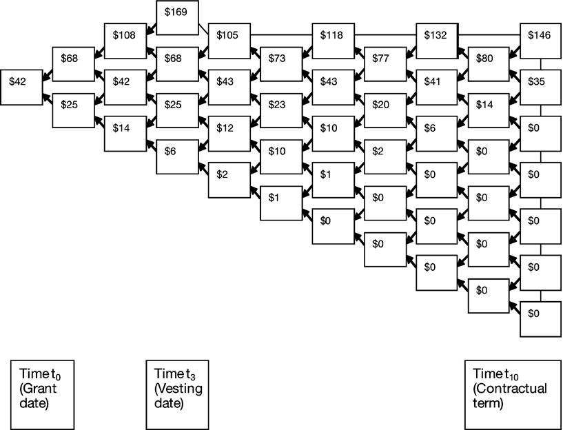
Figure SC 8-10 illustrates the adjusted calculation for the exercise multiple of 1.3 limited by the option's three-year vesting condition. This results in an exercise frontier with three segments—a vertical barrier at time t₃, to reflect the vesting condition, a horizontal barrier from t₃ to t₁₀, to reflect the exercise multiple of 1.3, and another vertical barrier at t₁₀, to reflect the contractual term of 10 years. If the stock price were to go to its highest possible node at the end of the second year (time t₂), the option would be exercised at the end of the next year, because the stock price will be above $130, with intrinsic value greater than $30 ($130 stock price minus $100 strike price) regardless of whether the stock price moves up or down from time t₂ to time t₃. The resulting calculation moves the estimated fair value to $34.56 (rounded to $35), very near to its estimated fair value in the original binomial lattice using a six-year static expected term (approximately $35.88, rounded to $36 in Figure SC 8-7).

Figure SC 8-10
Option tree—ten-year contractual term with a 1.3 assumed exercise multiple limited by the three-year cliff-vesting condition

View image

The results of the calculations in Figure SC 8-8, Figure SC 8-9 and Figure SC 8-10 are affected by the use of one-year time-steps in the lattice model. These time-steps are intended to illustrate the workings of the model. As noted earlier, a more realistic model would use shorter time intervals (e.g., daily) resulting in significantly more nodes. The model in Figure SC 8-7 with one-year time steps resulted in a valuation fairly close to the Black-Scholes value using a simple six-year expected term. In contrast, for the exercise assumptions in Figure SC 8-8, Figure SC 8-9 and Figure SC 8-10, a lattice model with smaller time intervals could produce values that differ by as much as 20% from those shown above. This is because the lattice values with the longer intervals may yield a stock price that well-exceeds an assumed exercise threshold in a single step when the option would theoretically be exercised at a lower price when shorter intervals are used. The values shown in the figures above are rough approximations illustrating the general relationship between results and model inputs with three-year cliff vesting and stock price volatility of 30%, as well as the exact calculations on a simplified basis (note the relationships will vary with different vesting schedules and volatility assumptions).

The examples shown above depict a constant exercise-frontier (except as affected by vesting or expiration of an option). In a more elaborate binomial model, the assumed early-exercise frontier may have a different slope or may be a probability distribution curve, rather than a straight line, that varies with both the price of the underlying stock and time. The binomial model can also incorporate additional assumptions regarding post-vesting cancellations, as discussed in SC 9.3.3.

For complex binomial models that reflect the correlation of stock price and early exercise, software applications may be employed to perform such modeling. As discussed further in SC 9.1, developing these models and the underlying assumptions manually will require considerable time and effort.

The lattice model also may be used to develop an implied expected term assumption, which is a required disclosure under ASC 718. The analysis of exercise patterns in a lattice model may yield an expected term that is shorter (or longer) than the expected term used in an otherwise similar Black-Scholes model. There are several methods to infer a single expected term from a lattice model, such as the method included in ASC 718-10-55-30, which solves for an implied expected term in the Black-Scholes model such that the Black-Scholes model's fair value equals the lattice model's fair value. Using this method, with an assumed exercise multiple of 2.0, the expected term assumption inferred in Figure SC 8-8 is approximately 8.2 years. Using the risk-neutral expected life method, the inferred expected term assumption is approximately 8.3 years. For typical options, the theoretical, inferred, risk-neutral expected term is much longer than the more realistic, and easily interpreted, implied Black-Scholes expected term.

There is a third method that would involve using a risk-adjusted expected rate of return in conjunction with early exercise assumptions built into the lattice model. The expected term assumption disclosed for companies using lattice models will therefore vary based upon the method used to infer it. The method used to infer the expected term should be applied consistently.

Because lattice models are flexible, they can accommodate a variety of situations and assumptions. Four specific adaptations of lattice models are:

When valuing options with service conditions only, the primary reason to use lattice models instead of the Black-Scholes model is to incorporate more detailed assumptions about employee exercise behavior. Companies considering whether to use a lattice model or the Black-Scholes model should consider their specific circumstances. For options on shares of a company with a relatively low stock price volatility and a longer vesting schedule, a simple lattice model may not yield a significantly more refined estimate of fair value than a Black-Scholes model using an appropriately developed weighted-average expected term assumption. Further, not all companies will have the necessary historical data required to support a more complex lattice model. These factors, taken together with the alternative to use a simplified method to calculate the expected term for "plain vanilla" options (as described in SC 8.4.1), may make the Black-Scholes model the more practical approach for valuing many "plain vanilla" options.

In general, the development of appropriate assumptions—inputs to the valuation model—is more critical than the model—Black-Scholes or lattice—for many typical option grants. SC 9 discusses the factors to be considered in the development of assumptions.

To understand various techniques for incorporating early exercise patterns into a lattice model, consider a simplification used in many of the illustrations that appear in ASC 718. The exercise of 100% of the options occurs when the underlying stock reaches a certain price. Using this assumption is similar to using a single value for the expected term, except that it assumes options are exercised when a specific stock price is reached, instead of after a specific time period. An appropriate lattice model, at a minimum, should capture early exercise patterns as a function of at least four factors: (1) the assumed exercise multiple(s), (2) the vesting period, (3) the contractual term, and (4) the assumed post-vesting termination rate(s). These factors replace the single expected term assumption that is used in the Black-Scholes model.

As described earlier, the exercise-multiple (or suboptimal exercise factor) is an assumption about early exercise behavior based on stock price appreciation rather than the time that has elapsed since the grant date. This factor is called suboptimal because traditional financial theory suggests that the optimum behavior is to hold an option until its contractual expiration date. Although suboptimal from a financial theory perspective, it may nevertheless be reasonable for an employee to exercise stock options early, given the fact that typical employee options cannot be sold or hedged and considering individual employee's risk tolerance, taxable income expectations, or liquidity needs. For example, a suboptimal exercise factor of 1.5 assumes that employees will voluntarily exercise options granted at-the-money when the price of the underlying stock price rises 50% above its price on the grant date. Typically, larger suboptimal exercise factors are associated with higher volatility stocks. Because of the sensitivity of an option's fair value to the early exercise assumption, it is particularly important that any suboptimal exercise factor in a lattice model be reasonable in the context of the specific company circumstances, the nature of the award, and the relevant employee demographics.

In addition to the other assumptions, lattice models should include an assumed post-vesting termination rate. Under most option plans, employees who terminate their employment have a short period (e.g., 90 days) to exercise their vested options. Lattice models typically assume that employees subject to truncation of the option's contractual term will exercise their options immediately upon termination if the options are in the money, and that out-of-the money options will always be cancelled upon termination.

To maximize the precision provided by a lattice model, more complex assumptions may need to be developed to reflect suboptimal exercise factors that change during the option's contractual term. For example, for an option with a three-year vesting provision and a ten-year contractual term, the assumed suboptimal exercise factor might be 1.8 in years 4-5, 1.5 in years 6-7, 1.4 in years 8-9, and 1.2 in year 10. Such an assumption reflects the notion that employees may demand larger payoffs to exercise options in the early years after grant but settle for less gain as the contractual term nears its end. Extending this concept even further, probability of early exercise can be added to the model to create a distribution of early exercise factors. For instance, in the above example for years 4-5, instead of assuming all employees will exercise when the stock price reaches 1.8 times the grant price, it could be assumed that, on average, one-third of the options will be exercised at a suboptimal exercise factor of 1.3, one-third at 1.6 and one-third at 1.9.

The following sections illustrate the use of suboptimal exercise factor(s) and the assumed post-vesting termination rate in a lattice model.

Figure SC 8-11 expands the binomial approach to reflect suboptimal exercise factors that change during the option's contractual term. This version of the lattice model uses a probability distribution of early exercises as it considers a scenario where employees would voluntarily exercise their options early (sub optimally) at stock price appreciation levels that vary by post-vesting sub-period. This distribution of early exercise patterns might be refined over time with the company's new grants to reflect the observed variance around the expected level of stock price appreciation that results in early exercise. Figure SC 8-11 illustrates an equally weighted probability distribution using three different suboptimal exercise factors for each of four post-vesting sub-periods.

This example assumes that employees will, on average, exercise one-third of the outstanding vested options on each trading day when the stock price is at least equal to the lowest suboptimal exercise factor, an additional one-third of the outstanding vested options will be exercised when the stock price is at least equal to the midpoint suboptimal exercise factor, and the remaining one-third will be exercised when the stock price is at least equal to the highest suboptimal exercise factor. This probability calculation occurs at each node of the lattice to simulate trading days. In other words, the assumption is that there is a 33% probability of early exercise of the outstanding vested options on the trading days when the stock price is between the lowest and middle suboptimal exercise-factors, a 67% probability of exercise when the stock price is between the middle and highest suboptimal exercise factors and a 100% probability if the highest stock price level has been reached. In addition, a small number of employees will be assumed to terminate employment after vesting, meaning their options will be exercised immediately (if in-the-money) or cancelled (if out-of-the money).

This example uses a much more detailed binomial lattice than was used in the previous examples (Figure SC 8-6, Figure SC 8-7, Figure SC 8-8, Figure SC 8-9 and Figure SC 8-10). In order to incorporate an early exercise assumption, the binomial model used with the assumptions shown below has 252 nodes per year (to reflect the number of market trading days in a year) over a full ten-year period, so there are approximately three million possible nodes, as opposed to the 28 nodes in Figure SC 8-7. 

Figure SC 8-11 illustrates a binomial model with probability-based exercise distributions of suboptimal exercise factors.

Figure SC 8-11
Binomial model with probability-based exercise distributions of suboptimal exercise factors

Monte Carlo techniques were used to simulate probability-based early exercise in Figure SC 8-11. The assumed suboptimal exercise factors decline over the option’s contractual term. This assumption is designed to replicate an effect observed by economists; namely, that employees may demand larger payoffs before voluntarily exercising their options when there is a longer time remaining in the contractual term for them to exercise. It is assumed that employees will exercise all in-the-money options by the expiration date. Figure SC 8-11 also assumes a constant post-vesting termination rate for simplicity.

Based on the assumptions in Figure SC 8-11, the binomial lattice model produces a fair value per option of $36.21. The increase over the fair value of $34.56 derived in Figure SC 8-10 based on a single suboptimal exercise factor of 1.3 reflects the higher suboptimal exercise factors in the earlier years from grant date (lower probability of early exercise). These fair values are both relatively close to the Black-Scholes model fair value for these options (as determined in Figure SC 8-5 using a 6-year expected term) of $35.29. For purposes of comparison, the implied expected term corresponding to this example equals 6.3 years. This implied expected term was calculated using the method described in ASC 718-10-55-30 (the expected term necessary for the Black-Scholes value to equal the lattice model value).

Companies should be cautious about using a single suboptimal exercise factor in their models, as they may underestimate fair value unless there is sufficient support for the assumption that there is a single level of price appreciation (measured as a proportion of exercise price) at which early exercise by employees tends to occur. However, a company will have difficulty either assessing reasonableness or estimating the effects of using various types of lattice models without developing such models—like the example in Figure SC 8-11—and doing the work necessary to develop and support appropriate assumptions. In the absence of a lattice model that incorporates complexities, such as probabilistic exercise, companies may be better served by using the Black-Scholes model with well-supported assumptions rather than attempting to implement a simplistic lattice model, especially for "plain vanilla" awards with longer vesting schedules.

The terms of some awards require that vesting or exercisability depend on achieving a market condition. For example, an option with a market condition may provide that the option cannot be exercised unless the stock price rises by 50% from the grant date price. Performance shares (generally, a promise to issue shares, or entitle employees to vest in share awards, if certain performance targets are met) may also contain market conditions. Awards with market conditions require the use of a lattice model or a Monte Carlo simulation to estimate fair value. For example, a restricted stock unit may contain a provision that vesting is contingent on the company's total shareholder return exceeding the total shareholder return of a specified peer group over a stated number of years.

Figure SC 8-12 illustrates an option that will vest only after the stock has traded at $150 or more for twenty consecutive trading days and the employee completes three years of service. The option will lapse if the stock does not reach its targeted price within three years of the grant date. The award includes a service condition and a market condition.

Figure SC 8-12
Option that vests after three years of service if a targeted stock price is achieved within three years

A Monte Carlo simulation or lattice model should be used to estimate the fair value of an option with this type of market condition because it is the only way to simulate the many possible ways stock prices can move to meet the targeted stock price.

Using a Monte Carlo technique with daily stock price intervals to simulate an appropriately large binomial model yields a fair value estimate of $24.26. This fair value estimate is considerably less than the valuations of similar options without a market condition (see Figure SC 8-6, Figure SC 8-7, Figure SC 8-8, Figure SC 8-9, and Figure SC 8-10).

On the other hand, the estimate of $24.26 is greater than the valuation that would result if the actual stock price had to be at or above the targeted stock price on a specific vesting date, for example, three years after grant (with otherwise similar assumptions as in Figure SC 8-12). These differences should be intuitive in that an option with a market condition is clearly worth less than an option that vests over the same time regardless of stock-price appreciation. Further, an option that can achieve the target stock price anytime during a three-year period offers the holder greater flexibility (possible early vesting, with potential gains in the case of early stock-price appreciation) and thus should be worth more than an option that vests only if the stock price is at or above its target price upon completion of three years of service.

Other assumptions in the valuation model for awards with market conditions should be tailored to reflect the award's terms. For example, in Figure SC 8-12, because the options vest based on stock price movements, using a single expected term assumption would not be reasonable. Rather, a lattice model or Monte Carlo simulation is needed to reflect the fact that exercise could occur early if the stock price reaches $150 relatively early in the required three-year service period. The model uses a simplified exercise assumption of three and one-half years after achieving the target stock price to reflect the contingent nature of the vesting date and a typical holding period after vesting. More refined early exercise assumptions could also be appropriate.

A lattice model or Monte Carlo simulation should also be used to value an award that involves the achievement of multiple possible market conditions. For example, an option that will vest if the share price doubles within the next two years or if it triples within the next five years and the employee stays with the company until either condition is met should be viewed as one award, with a fair value determined by a lattice model or Monte Carlo simulation.

Market conditions are typically modeled using an approach that incorporates a Monte Carlo simulation (involving a series of random trials that may take different future price paths over the award's contractual life based on appropriate probability distributions). Conditions are imposed on each Monte Carlo simulation to determine if the market condition would have been met for the particular stock price path. For example, in modeling the market condition in Figure SC 8-12, each simulated stock price path was checked to determine whether the stock reached the $150 threshold during the vesting period.

The point at which the stock price achieves the threshold in each scenario in the simulation is also important in determining fair value. This technique for modeling awards with market conditions is called path-dependent modeling because it simulates many possible stock price paths through the lattice (or simulation) to arrive at the outcome. The award's measurement date fair value is determined by taking the average of the measurement date fair values under each of the scenarios in the Monte Carlo simulation.

In addition, the median path of successful trials for the market condition is used to develop the derived service period (as described in SC 2). The pattern of expense recognition will depend on this value in many cases (see SC 2.6.2 for more details).